EWA Volume Splatting
elliptical Gaussian kernels 椭圆高斯核
Splatting algorithms interpret volume data as a set of particles that are absorbing and emitting light. 泼溅算法将体素数据解释为一组吸收和发射光的粒子。
Our method is based on a novel framework to compute the footprint function, which relies on the transformation of the volume data to so-called ray space. This transformation is equivalent to perspective projection. By using its local affine approximation at each voxel, we derive an analytic expression for the EWA footprint in screen space. The rasterization of the footprint is performed using forward differencing requiring only one 1D footprint table for all reconstruction kernels and any viewing direction.”
我们的方法基于一个新的框架来计算足迹函数,该框架依赖于将体积数据转换为所谓的射线空间。这种转换相当于透视投影。通过在每个体素处使用其局部仿射近似,我们推导出了屏幕空间中EWA足迹的解析表达式。足迹的光栅化是使用正向差分进行的,只需要一个1D足迹表用于所有重建内核和任何观察方向。

Splatting Algorithms

a point in ray space:
The coordinates $x_0$ and $x_1$ specify a point on the projection plane.
The ray intersecting the center of projection and the point $(x_0,x_1)$ on the projection plane is called a viewing ray.
The third coordinate $x_2$ specifies the Euclidean distance from the center of projection to a point on the viewing ray.
The volume rendering equation:
$g(x)$ is the extinction function that defines the rate of light occlusion, and $c_λ(x)$ is an emission coefficient.
$c_λ(x)g(x)$ is also called the source term,describing the light intensity scattered in the direction of the ray $x$ at the point $x_2$.
coefficients $g_k$ and reconstruction kernels $r_k(x)$
We also assume that the emission coefficient is constant in the support of each reconstruction kernel along a ray, hence we use the notation $c_{λk}(x)=c_λ(x,x_2)$
approximate the exponential function with the first two terms of its Taylor expansion, thus $e^x≈ 1−x$.
The EWA Volume Resampling Filter
Aliasing in Volume Splatting
achieve this band-limitation by convolving $ I_λ(\hat{x})$ with an appropriate low-pass filter $ h(\hat{x})$, yielding the antialiased splatting equation:
First, we assume that the emission coefficient is approximately constant in the support of each footprint function $q_k$, hence $c_λk (\hat{x}) ≈ c_λk$ for all $\hat{x}$ in the support area.
Together with the assumption that the emission coefficient is constant in the support of each reconstruction kernel along a viewing ray, this means that the emission coefficient is constant in the complete 3D support of each reconstruction kernel.
Additionally, we assume that the attenuation factor has an approximately constant value $o_k$ in the support of each footprint function:
ideal resampling filter,footprint function $q_k$ and a low-pass kernel $h$
This means that instead of band-limiting the output function directly, we band-limit each footprint function separately.
Elliptical Gaussian Kernels
We define an elliptical Gaussian $G_V(x − p)$ centered at a point $p=(p_0,p_1,p_2)^T$ with a variance matrix $V$ as:
$x=(x_0,x_1,x_2)^T$
the affine mapping as $Φ(x)= Mx + c$, where $M$ is a 3 × 3 matrix and $c$ is a vector $(c_0,c_1,c_2)^T$ . We substitute $x =Φ^{−1}(u)$ in (9), yielding:
convolving two Gaussians with variance matrices $\bf{V}$ and $\bf{Y}$ results in another Gaussian with variance matrix $\bf{V + Y}$:
integrating a 3D Gaussian $\mathcal{G}_V$ along one coordinate axis yields a 2D Gaussian $\mathcal{G}_{\hat{V}}$, hence:
where $\hat{\bf{x}} =(x_0,x_1)^T$and $\hat{\bf{p}} =(p_0,p_1)^T$ . The 2 × 2 variance matrix $\hat{\bf{V}}$ is easily obtained from the 3 × 3 matrix $\bf{V}$ by skipping the third row and column:
The Viewing Transformation
object space, which has coordinates $\bf{t}=(t_0,t_1,t_2)^T$ ,the Gaussian reconstruction kernels in object space:
camera coordinates : $\bf{u} =(u_0,u_1,u_2)^T$,Object coordinates are transformed to camera coordinates using an affine mapping $\bf{u} = φ(\bf{t})$, called viewing transformation:
We transform the reconstruction kernels $\mathcal{G}_{V^{′′}_k} (\bf{t} − \bf{t}_k)$to camera space by substituting $\bf{t} = φ^{−1}(\bf{u})$ and using Equation (10):
where$\bf{u}_k = φ(\bf{t}_k)$ is the center of the Gaussian in camera coordinates and $r^{‘} _k(\bf{u})$ denotes the reconstruction kernel in camera space.the variance matrix in camera coordinates $V^{′}_k$ is given by $\bf{V}^{′}_k = \bf{WV}^{′′}_k\bf{W}^T$ .
The Projective Transformation
Camera space and ray space are related by the mapping $\bf{x = m(u)}$:
where $ l=|( x_{0}, x_{1}, 1 )^{T} |$.
the local affine approximation $\bf{m}_{u_{k}}$ of the projective transformation. It is defined by the first two terms of the Taylor expansion of $\bf{m}$ at the point $\bf{u}_k$:
apply Equation (10)


Integration and Band-Limiting
Gaussian footprint function $q_k$:
Gaussian low-pass filter:
EWA volume resampling filter:
Reduction from Volume to Surface Reconstruction Kernels

As s approaches infinity, we therefore get the following 2D variance matrix $\hat{\bf{V}}$:

 微信
微信 支付宝
支付宝